Forecasting GDP in the presence of breaks: when is the past a good guide to the future?
George Kapetanios, Simon Price and Sophie Stone.
Bank of England, 20 August 2015
Structural breaks are a major source of forecast errors, and few come larger than the recent financial crisis and subsequent recession. After a break, formerly good models stop working. One way to cope is to discount the past in a data driven way. We try that, and find that shortly after the crash it was best to ignore almost all data older than three years – but now it is again time to take a longer view.
Introduction
It is often argued (eg by Clements and Hendry) that structural change is the main cause of forecast errors. Often this appears as an apparent break in the unconditional mean (eg long-run GDP growth), even if the true change lies elsewhere. The period since the financial crisis is an obvious example – few foresaw the depths of recession, or the size of the apparent drop in productivity growth.
You might think that after a break has happened you can simply switch to a new model. But break detection is hard in real time, and even if you knew for sure that a break has just occurred, you would still want to use some pre-break data to estimate the model. This follows from the familiar mean-variance trade off – using only post-break data reduces bias (helps you estimate the mean correctly) but as there is little data available at first, estimation uncertainty is large (increases the variance). For known breaks, Pesaran and Timmerman advocate combining models estimated over many different sample periods, spanning the break.
But usually we don’t know if there has been a break, so one approach is to use models that are robust to them. Generally, discounting the past is a good way to go. In Giriatis, Kapetanios and Price a data-dependent method of picking the optimal discount factor is explored, based on past evidence of forecast performance. This method has good properties for many types of structural change and can be implemented using a variety of approaches. In the rest of this post we show how some approaches perform in a real and important example.
A recent (but historically infrequent) case in point
After the financial crisis, arguably a less than once in a century event, and subsequent recession, forecasters around the world started making enormous forecast errors. The Bank of England was no exception, in both inflation and (on which we focus here) GDP growth.
The forecasts published in the Inflation Report belong to the MPC, but the staff maintain a ‘statistical suite’ of non-structural models to forecast GDP growth and inflation which are used to provide an agnostic cross-check on the MPC’s forecasts. They make no assumptions about the structure of the economy and are judgement-free. In the earliest version, breaks (primarily in inflation) were handled by trying to detect them statistically, and then forecasting the ‘demeaned’ data by subtracting the estimated averages. Subsequently those forecasts moved to a simple robust method: a short ‘rolling’ estimation window where the length of the estimation sample is fixed and moves on by one quarter every period (as opposed to the sample increasing as time goes by). But although based on some investigation, the choice of window length was pretty arbitrary and fixed at seven years.
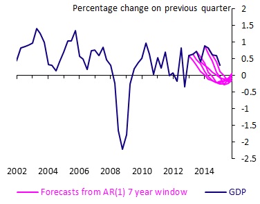
The sharp falls in GDP during the crisis soon dominated the estimation sample. As most of the models in the suite have forecasts that tend to revert back to the sample mean fairly rapidly, they consequently did relatively well after the recession first hit because they quickly factored in slower growth. But when GDP growth recovered in 2013-14 they consistently under-predicted. This includes the ‘low-order’ autoregressive (AR) model (ie where growth is regressed solely on a small number of its own lagged values), which often performs well and is a common forecast benchmark. This is neatly illustrated in Figure 1 with the successive forecasts from an AR(1) model (ie with one lag), estimated using a seven year window. The forecasts all converge to a low value.
So could these forecasts have been improved if they had used data-dependent methods to determine window length or, more generally, to discount the past?
Finding the best window
Here we explore three approaches.
One is to optimise the length of the rolling estimation window, based on recent forecast performance. This is relatively extreme – past data within that window is given 100% weight but any data before the window starts is ignored.
A second, more natural approach might be to include all available data and place less weight on older observations than more recent observations. The Exponentially Weighted Moving Average (EWMA) of past data is one popular and simple way to do this.
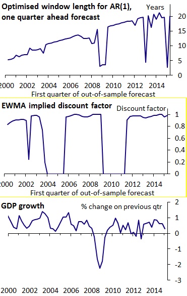
For the AR, as the potential sample increases the maximum possible window increases. But as Figure 2 shows (with GDP growth in the bottom panel for reference), the optimal AR(1) window length fell from around 15 years to three years during the crisis. Similarly, the discount factor fell very rapidly from close to unity (don’t discount past data – use the whole sample) to zero (just use the most recent observation available), and stayed there. That effectively means we would have had a random walk (no-change) forecast, where the forecast is whatever the previous observation was. Consistent with this finding, the suite tended to give a large weight to the random walk model during the recession. That method will perform well after a major break, although may not be so good in normal times. After 2011, the optimal weight quickly rose towards unity again. So both these methods suggest that older observations should have received little or no weight for forecasting GDP during and (in the case of the EWMA) immediately post-crisis, and that we should now again place more weight on older observations.
And this would have helped. The Table shows a measure of forecast performance, Root Mean Square Forecast Error (RMSFE); the smaller the number, the better the performance. Using GDP data from 1990Q1 onwards, the forecasts are produced in ‘pseudo-real time’. This means that they take no account of data revisions, but more importantly, only data for periods prior to the forecast period are used (ie, taking account of publication dates). They are direct forecasts, so that if we want to forecast GDP (eg) four periods ahead, instead of forecasting one-step ahead and then iterating forward to generate forecasts at longer horizons, we run a regression directly on GDP led four periods. Both the optimised-window AR(1) and the EWMA use ‘cross-validation’, in which forecast performance in one part of the sample is used to determine the parameters in another part of the sample – in this case, the rate at which the past is discounted for predicting GDP in a given quarter is determined by forecast performance in the previous ten quarters. As can be seen in the first two rows, an AR(1) with a seven-year window actually performs reasonably well relative to an optimised-window AR(1) and the EWMA for forecasting GDP in the whole period (2002-2014). But it performed worse in 2014, particularly at longer horizons.
It could the state, not the time, that matters
The third ’non-parametric‘ approach does not assume any particular shape for the weight function, unlike the EWMA, and in particular does not impose monotonically declining weights on past data. This could be useful because different stages of the cycle have different properties, and some past periods are likely to be better guides to the future than others. So when forecasting GDP during recovery periods, placing higher weights on observations during previous recoveries may produce a better forecast.
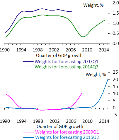
Figure 3 shows the weights this approach would place on each previous quarter of GDP growth (on the x-axis), to forecast GDP growth at a particular point in time. There is nothing to stop weights from being negative, but where that happens they are small. At 2007Q1, they are similar to those of a relatively long window. But by 2009Q1, during the crisis, it would have suggested placing most weight on the most recent observations and the recession period in 1990-91, while ignoring periods of economic expansion. Then for forecasting GDP in the recovery (from 2014Q1 onward) it would have put little weight on the crisis period and the recession in the 1990s. And it now places almost full weight on the recent recovery period.
Conclusions
Forecasters need strategies for forecasting in the presence of breaks in their toolkit. No single approach consistently performs best at all times. A benchmark AR model with a very short estimation window for forecasting UK GDP worked well during the crisis, but over the past year a long estimation window did better.
A key issue not only for forecasting but also for policy is whether the structural change is permanent. That hugely important question is beyond the scope of this blog piece. All this piece can say is that in a world of recurring structural change it is a good idea to keep an eye on robust forecasts that discount the past in a data-dependent way.
George Kapetanios works at Queen Mary University of London, Simon Price works in the Bank’s Monetary Analysis Division and Sophie Stone works in the Bank’s Conjunctural Assessment and Projections Division.
Bank Underground is a blog for Bank of England staff to share views that challenge – or support – prevailing policy orthodoxies. The views expressed here are those of the authors, and are not necessarily those of the Bank of England, or its policy committees.
If you want to get in touch, please email us at bankunderground@bankofengland.co.uk


