
Unraveling the Oil Conundrum: Productivity Improvements and Cost Declines in the U.S. Shale Oil Industry
Ryan Decker, Aaron Flaaen, and Maria Tito
FRB, March 22, 2016
Oil prices have declined by roughly 70 percent since peaking in the middle of 2014. The U.S. oil rig count–a common measure of drilling activity–peaked in late 2014 and has since declined by about 60 percent. Yet U.S. production of crude oil continued rising until the middle of 2015 and has since fallen by only 6 percent from its peak. The dramatic advance of U.S. oil production seen in the last decade–driven primarily by new discoveries of shale oil and innovation in drilling and extraction technology–has not been as responsive to the deterioration of oil markets as some analysts predicted.2
Why have large declines in prices and in the rig count not triggered a more dramatic decline in production? At what price level would a large share of U.S. shale oil production lose economic viability? In this note, we explore these questions with a focus on the U.S. shale oil industry in the Bakken, Eagle Ford, and Permian Basin regions.3 We describe large productivity improvements in drilling and fracking methods that have allowed production to remain strong despite falling rig usage. We then document cost declines that have preserved profitability for many firms even in the midst of historically low prices.
The Resilience of Production
The dramatic increase in total U.S. oil extraction between 2011 and mid-2015 was driven almost entirely by unconventional production in geologies such as shale; these areas now account for more than half of U.S. output. The recent decrease in extraction has likewise been concentrated in unconventional production.4 This decline has been moderate in light of the large collapse in prices and in the rig count. One explanation for the modest response of production to the deterioration of the oil market is the high pace of productivity growth seen by the shale extraction industry in recent years.
| Figure 1. Rig Counts and Wells per Rig, Bakken Region |
|---|
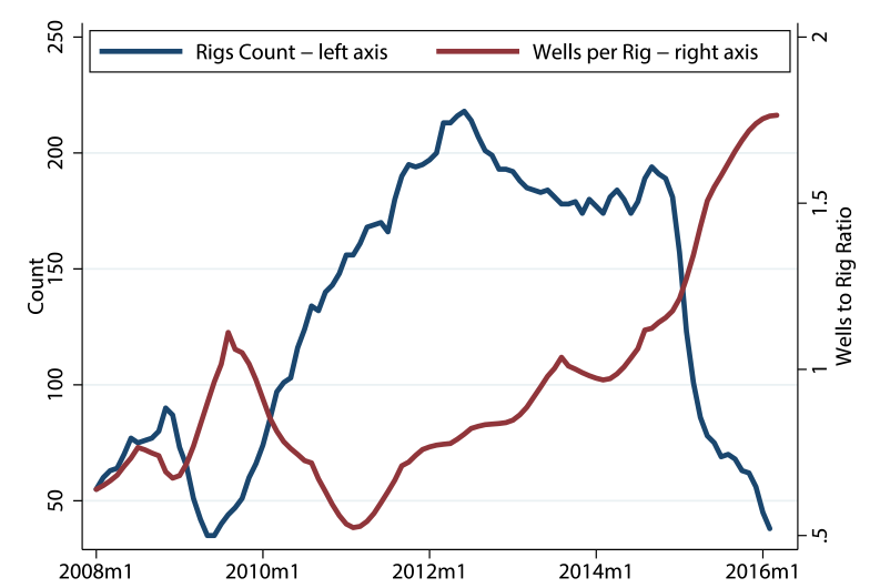 |
Improvements in the number of wells a rig can drill each month and in the average length of each well have contributed to the productivity gains in drilling. As shown in Figure 1, which plots data for the Bakken region, the number of wells drilled per rig in a given month has risen steadily since 2011, and it accelerated further after the rig count began falling in 2014.5The main driver of this greater rig efficiency is the adoption of pad drilling technology whereby a rig can drill multiple wells from the same spot without the need for expensive and time-consuming disassembly, relocation, and reassembly. Additionally, each well has become much larger, as the average well length has doubled from roughly one to two miles (American Petroleum Institute (API) 2015, Quarterly Well Completion Report. IHS Global Inc.).
Increased and more efficient use of water, sand, and other proppants in the fracking process has further enhanced the productivity of oil wells, particularly early in the well lifecycle.6 As a result, in addition to the increase in the number of new wells per rig, the extraction from these new wells in their first month of production has roughly tripled since early 2008.7These improvements can be best illustrated by examining well decline curves, which track productivity over a well’s lifecycle.
| Figure 2. Average Well Decline Curve by Cohort |
|---|
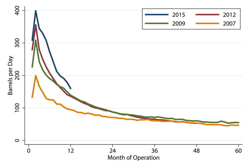 |
To facilitate a more disaggregated analysis, we use well-level data for the Bakken region from the North Dakota Department of Mineral Resources. These data provide monthly production by well in addition to other well characteristics and account for roughly 95 percent of total Bakken oil production. Figure 2 plots well decline curves for selected well cohorts, defined by year of drilling, in the Bakken region. The y-axis reports average well output in barrels per day. The x-axis tracks months of operation–the well lifecycle. The changes in productivity of wells in early months of production are striking: output during the first full month of production has roughly doubled since 2007. The series of upward shifts in productivity paths seems to persist throughout the lifecycle across subsequent well cohorts. While innovations in fracking technology are primarily thought to shift production forward in the well lifecycle (rather than to increase total lifetime output), well-level data suggest that output in later-producing months has actually increased in recent years.
| Figure 3. Well Decline, Controlling for Well Size |
|---|
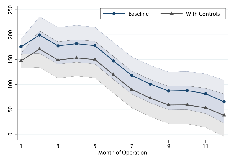 |
How much of this increase in productivity is driven solely by expansions of well size, as opposed to innovations in fracking technology? Using data for the Bakken region, we regress well-level output on a series of monthly indicators that are distinct for each cohort year. The resulting cohort-specific well-decline coefficients capture the change in output along each month of operation compared to a baseline year, for which we choose 2007. The coefficients for the cohort of 2015 are shown in blue in Figure 3. (Notice they are roughly equal to the difference in the well decline curves between 2015 and 2007 in Figure 2.) Next, we add a measure of well size to the regression, specifically, the lateral distance of a well that undergoes perforations in preparation for fracking. As shown in grey in Figure 3, these adjusted coefficients are not largely different from the raw coefficients without the well-size adjustment. This analysis points to innovations apart from increases in well size as the main contributing factors to the output gains evident from Figure 2.
| Figure 4. Decomposition of Production Changes |
|---|
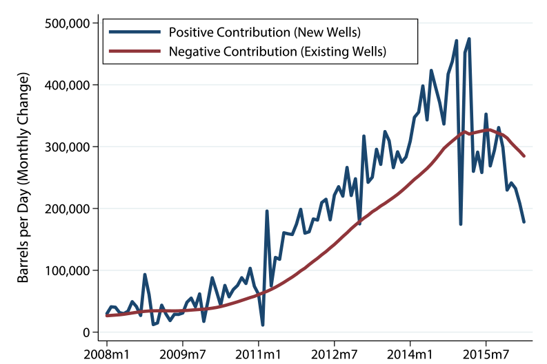 |
Other lifecycle and composition issues can provide further insights into aggregate production. Figure 4 decomposes the change in monthly oil production from all regions into the positive contribution of new wells (the blue line) and the negative contribution from existing wells (the red line), the latter being almost invariably negative as a result of the natural lifecycle declines depicted in Figure 2. Consequently, aggregate production increases whenever output from new wells (the blue line) exceeds the natural output declines among existing wells (the red line). Despite productivity improvements, output from new wells began falling in mid-2015 as the number of well completions dropped significantly. This pushed the positive contribution from new wells below the negative contribution from existing wells, resulting in aggregate production declines. It is noteworthy, though, that the drag from existing well declines peaked shortly thereafter, mitigating the fall in aggregate output. Completions of larger wells and productivity improvements among legacy wells have softened the negative pull from existing wells.
| Figure 5. Rigs Needed for Flat Production |
|---|
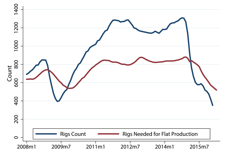 |
Figure 5 provides another way of understanding composition effects behind production, the number of rigs needed to maintain a constant production level, that is, rigs needed for flat production (RNFP). This measure is constructed by calculating the number of new rigs necessary to offset observed declines from existing wells, using the prior month’s estimate of new production per rig. As rig efficiency has increased and legacy-well decline curves have shifted up, and as total production has gradually fallen, the RNFP has declined. This framing highlights a decreasing usefulness of the rig count as a sole indicator of overall activity.
General equilibrium mechanisms have also affected the oil production climate. Lower drilling activity combined with productivity enhancements have reduced the demand for workers, and wages of workers in the Natural Resources and Mining sector have declined by 10 percent or more in the three main shale regions.8 Service costs have fallen by about 30 percent in the shale regions (Curtis 2015), with anecdotal reports even indicating that some service firms are performing tasks for free to retain market share. Diesel fuel and other energy sources are key production inputs, and their costs have fallen mechanically with oil prices. Using cost share estimates from the Energy Information Administration (EIA) from 2009, we construct a back-of-the-envelope estimate that labor, services, and fuel cost reductions have collectively reduced overall production costs by more than 10 percent.9 Other costs have fallen with broad market conditions as well, most notably royalties and taxes (which often depend nonlinearly on prices).10
Additional productivity improvements and cost reductions have resulted from the aggressive reallocation of drilling and operating activity toward high-productivity plays and rigs as well as from the failure or acquisition of low-productivity, high-cost firms.11 Considering the recent productivity improvements, how should we expect aggregate production to evolve in coming months and years? The EIA, accounting for the various productivity and lifecycle factors described above, forecasts total U.S. oil production to gradually fall to about 8.2 million barrels per day in early-2017, flattening out thereafter (U.S. Energy Information Administration 2016b).
Economic Viability of Shale Production
In recent years, companies have made extensive efforts to reduce drilling and production costs. Cost estimates vary widely, reflecting substantive variation in regional and company-specific costs, ambiguity about the details of cost estimation, and general uncertainty. Our goal is to generate a range of estimates that can inform our view of the economic viability of continued shale oil production.
We focus on two important cost types. The first are often referred to as “cash costs”, and for our purposes they include the costs of operating a lease (such as pumping, equipment rental, servicing, and materials) as well as administrative costs and per-barrel taxes. Roughly speaking, these can be thought of as the average per-barrel cost of ongoing production at existing wells. At the margin, production from an existing well is profitable so long as prices can cover cash costs and transportation expenses. The second cost measure is the long-cycle breakeven, an estimate of the oil price that would make new drilling profitable. The long-cycle breakeven can be thought of as the cost that is most relevant to long-term production growth.
Publicly traded oil companies report cash costs to the SEC in quarterly and annual filings. We collected these costs from 10K reports for 2013 and 2014. We also obtained the costs for the first nine months of 2015 from 10Q reports. We use data for about 25 companies with large operations in the three main shale regions and that focus primarily on oil production.12We report these costs in Figure 6.
| Figure 6. Cash Costs |
|---|
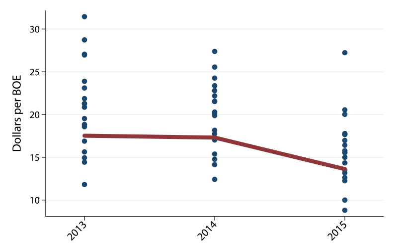 |
Each blue dot in Figure 6 represents a firm, and the red line shows the production-weighted average across companies. The weighted average includes all companies for which we have all three years of data, though some small, high-cost companies are omitted from the scatter. Figure 6 shows that cash costs vary widely across companies; various sources also indicate wide cost dispersion across wells within firms. The between-firm dispersion has declined some over time, as has the average cost, falling from about $18 per barrel to about $14 per barrel (without considering survivorship bias). The decline represents both aggressive cost-reduction efforts by firms and the general equilibrium cost reductions discussed above. With transportation costs ranging from $5 to $10 (depending on region and resources), the data suggest that for many firms the cost of operating existing wells is still somewhat below the current oil spot price.
| Figure 7. Long-Cycle Breakeven Estimates |
|---|
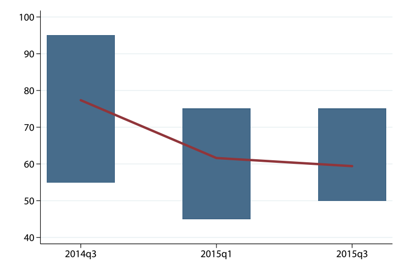 |
In the longer term, an important cost threshold is the long-cycle breakeven. This threshold includes drilling and transportation costs (as well as internal cost of capital hurdles) and therefore reflects the price at which new wells are economically profitable. Estimates of long-cycle breakeven costs vary widely. In Figure 7, we report results from quarterly surveys of oil companies administered by the Federal Reserve Bank of Kansas City (and, as such, include operations primarily in the Niobrara region). Respondents were asked to name the price at which new drilling could be expected to be profitable. Each bar captures the overall distribution of breakeven prices reported in each quarter (we only include firms that responded in all three time periods). As in Figure 6, the red line represents the average across firms (in this case we use a simple average since production data are not available from the survey).
Again, there exists wide variation in costs across companies. But, as with cash costs, dispersion has narrowed some, and average costs have fallen significantly since 2014. Breakeven prices averaged about $60 per barrel in the third quarter of 2015. Given the pace of cost reduction, by early 2016, costs are likely to have declined further. Estimates for other regions tend to be somewhat lower as well. Table 1 reports long-cycle breakeven estimates from a variety of sources.13
| Table 1. Breakeven Estimates |
|---|
| Region | Date | Source | Estimate |
|---|---|---|---|
| Bakken | 2015q3 | NDIC | $30-$45 |
| Bakken | 2015q3 | Minn. FRB | $53 |
| Eagle/Permian | 2016q1 | Bloomberg Intelligence | $23-$59 |
| Niobrara | 2015q3 | KC FRB | $60 |
| Multiple regions | Recent | Wells Fargo | $25-$46 |
| All regions | Recent | Rystad Energy | $36 |
Wells Fargo and Bloomberg Intelligence provide estimates for some regions that go as low as the mid-$20 range. Other regions have costs approaching $60. The estimates suggest that current prices are too low for much long-term economic viability of shale oil production. Given the lifecycle curves shown in Figure 2, aggregate production is not likely to remain strong or rise again until the market sees substantial price growth.
Simple marginal cost reasoning has limits in this industry. There is considerable anecdotal evidence that firms may choose to temporarily operate at prices below their costs for a variety of reasons. Many firms bought price hedges that have allowed them to continue selling some oil above spot prices, though some of these contracts will expire by the end of 2016. Shut-in costs–the costs of shutting down producing wells–are significant. Some firms may choose to operate below cost to retain market share or a core of skilled workers, to maintain cash flow for debt servicing or dividends, or to avoid losing production rights under certain types of lease terms.
Some firms may have continued ability to survive on credit, though this option may be running out. Oil company bonds are trading at large spreads, there have already been waves of defaults, and new issuance is down. Banks that lend to oil producers accept proven reserves as collateral, but periodically this collateral is marked to market. By mid-2015, U.S. onshore producers were devoting an average of 80 percent of cash flow to debt servicing costs (U.S. Energy Information Administration 2015). While outside the scope of the present study, these financial issues are likely to be a major driver of producer dynamics going forward. Financial markets may also be a mechanism that transmits oil market deterioration to the broader economy.14
In summary, the lack of a large production response to falling prices is likely due primarily to both rapid productivity gains and steadily falling costs of drilling and production. Additionally, aggressive reallocation efforts by firms have provided further boosts to aggregate productivity. While some of the factors boosting production–such as reallocation and labor hoarding–are likely to be temporary, other factors represent permanent improvements in exploration and drilling methods. These productivity improvements have led to considerable declines in cash costs for operating wells, and in breakeven thresholds for new wells. These costs may yet fall further. However, current breakeven estimates are generally higher than spot prices, suggesting that production growth may be muted for some time.
References
American Petroleum Institute. 2015. Quarterly Well Completion Report 31(4). IHS Global.
Bokowy, Tom and Ryan Hatcher. 2015. “ND Bakken Tax Trigger: Per Barrel Impact.” The Bakken Magazine March 3, 2015. At http://thebakken.com/articles/1029/nd-bakken-tax-trigger-per-barrel-impact (accessed March 14, 2016).
Cakir Melek, Nida. 2015. “What Could Lower Prices Mean for U.S. Oil Production?” Federal Reserve Bank of Kansas City Economic Review First Quarter 2015. Athttps://www.kansascityfed.org/~/media/files/publicat/econrev/econrevarchive/2015/1q15wcakirmelek.pdf  (accessed March 14, 2016).
Carroll, Joe. 2016. “Texas Shale Drillers Lure $2 Billion in New Equity to Permian.” BloombergBusiness February 1, 2016. At http://www.bloomberg.com/news/articles/2016-02-02/texas-shale-drillers-lure-2-billion-in-new-equity-to-permian (accessed March 14, 2016).
Curtis, Trisha. 2015. “US Shale Oil Dynamics in a Low Price Environment.” The Oxford Institute for Energy Studies paper no. WPM 62. At https://www.oxfordenergy.org/wpcms/wp-content/uploads/2015/11/WPM-62.pdf (accessed March 14, 2016).
The Economist. 2016. “The Oil Conundrum.” January 23, 2016. The Economist. At http://www.economist.com/news/briefing/21688919-plunging-prices-have-neither-halted-oil-production-nor-stimulated-surge-global-growth (accessed March 14, 2016).
Egan, Matt. 2016. “Big Banks Brace for Oil Loans to Implode.” CNN Money January 17, 2016. At http://money.cnn.com/2016/01/18/investing/oil-crash-wall-street-banks-jpmorgan/ (accessed March 15, 2016).
The Federal Reserve Bank of Kansas City. “Energy Survey.” Athttps://www.kansascityfed.org/research/indicatorsdata/energy (accessed March 14, 2016).
Glazer, Emily. 2016. “J.P. Morgan Sounds Fresh Warning on Energy-Loan Losses.” The Wall Street Journal February 23, 2016. At http://www.wsj.com/articles/j-p-morgan-sounds-fresh-warning-on-energy-losses-1456243537 (accessed March 14, 2016).
Grunewald, Rob. 2016. “From Red-Hot to Lukewarm in the Bakken.” Federal Reserve Bank of Kansas City fedgazette. January 28, 2016. At https://www.minneapolisfed.org/publications/fedgazette/from-red-hot-to-lukewarm-in-the-bakken (accessed March 14, 2016).
Loder, Asjylyn. 2016. “Shale Faces March Madness as $1.2 Billion in Interest Comes Due.” BloombergBusiness February 18, 2016. At http://www.bloomberg.com/news/articles/2016-02-18/shale-faces-march-madness-as-1-2-billion-in-interest-comes-due (accessed March 14, 2016).
Petroff, Alana and Tal Yellin. 2015. “What It Costs to Produce Oil.” CNN Money. At http://money.cnn.com/interactive/economy/the-cost-to-produce-a-barrel-of-oil/index.html?iid=EL (accessed March 14, 2016).
Pioneer Natural Resources. 2014. 2014 Annual Report. At http://investors.pxd.com/phoenix.zhtml?c=90959&p=irol-reportsAnnual (accessed March 14, 2016).
Raine, Chris. 2016. “U.S. Shale Still Covers Production Costs at $30 Oil.” Oil Daily, Energy Intelligence Group, February 11, 2016.
U.S. Energy Information Administration. 2010. “Oil and Gas Lease Equipment and Operating Costs 1994 through 2009.” September 28, 2010. Athttp://www.eia.gov/pub/oil_gas/natural_gas/data_publications/cost_indices_equipment_production/current/coststudy.html(accessed March 14, 2016).
U.S. Energy Information Administration. 2015. “Debt Service Uses a Rising Share of U.S. Onshore Oil Producers’ Operating Cash Flow.” Today in Energy September 18, 2015. At https://www.eia.gov/todayinenergy/detail.cfm?id=22992(accessed March 14, 2016).
U.S. Energy Information Administration. 2016. Drilling Productivity Report March. At https://www.eia.gov/petroleum/drilling/(accessed March 14, 2016).
U.S. Energy Information Administration. 2016. Short-Term Energy Outlook March. At http://www.eia.gov/forecasts/steo/(accessed March 14, 2016).
1. We thank Travis Adams, Emily Wisniewski, and Morgan Smith for excellent research assistance. Mine Yucel of the Federal Reserve Bank of Dallas and Rob Grunewald of the Federal Reserve Bank of Minneapolis each provided several helpful conversations and data. Jason Brown, Nida Cakir Melek, and Chad Wilkerson of the Federal Reserve Bank of Kansas City shared extensive background information, insights, and data of relevance to shale oil economics. We thank Deepa Datta, Rob Vigfusson, and Gustavo Suarez for several helpful conversations. Finally, Kim Bayard and Norm Morin provided extensive resources and guidance for this project. Return to text
2. One notable exception is Cakir Melek (2015) which stated that “even with a 50 percent decline in rig counts [in calendar year 2015], improvements in efficiency could increase production in 2015.” Return to text
3. The output from the Bakken, Eagle Ford, and Permian regions accounts for more than 85 percent of total production of shale oil. Return to text
4. Unconventional production, which now represents 55 percent of total output, amounted to 5.0 million barrels per day (mbd) in February 2016, down from the peak of 5.5 mbd in March 2015. Conventional production has instead oscillated around 4 mbd over the last year (U.S. Energy Information Administration 2016a). Return to text
5. U.S. Energy Information Administration (2016a). Return to text
6. See, for example, The Economist (2016). Return to text
7. The data refer to all regions of unconventional production as reported by the U.S. Energy Information Administration (2016a). Return to text
8. Data are from the Bureau of Labor Statistics’ Quarterly Census of Employment and Wages (QCEW). Region-level wages are computed as the employment-weighted average of county-level average weekly wages. Following Grunewald (2016), the Bakken region comprises the following counties: Billings, Burke, Divide, Dunn, Golden Valley, McKenzie, Mountrail, Stark, Williams, Richland, Roosevelt, and Sheridan. We define Eagle Ford and Permian Basin regions using county lists from the Railroad Commission of Texas. The Eagle Ford region included the following counties: Atascosa, Bastrop, Bee, Brazos, Burleson, De Witt, Dimmitt, Fayette, Frio, Gonzales, Grimes, Karnes, La Salle, Lavaca, Lee, Leon, Live Oak, Madison, Maverick, McMullen, Milam, Robertson, Walker, Webb, Wilson, and Zavala. The Permian Basin includes the following counties: Andrews, Borden, Cochrane, Coke, Crane, Crosby, Dawson, Dickens, Ector, Gaines, Garza, Glasscock, Hale, Hockley, Howard, Irion, Jeff Davis, Kent, Kimble, Lamb, Loving, Lubbock, Lynn, Martin, Midland, Mitchell, Nolan, Pecos, Reagan, Reeves, Scurry, Sterling, Terry, Tom Green, Upton, Ward, Winkler, and Yoakum. Return to text
9. The EIA Cost Study was discontinued after 2009. Using QCEW data for Natural Resources and Mining wages in Bakken, Eagle Ford, and Permian Basin data, we estimate that labor costs have fallen by about 10 percent. Our service cost estimate is based on the numbers suggested by Curtis (2015). According to EIA, per-gallon diesel prices fell from $3 to $1.84 during 2015 (STEO date), or by more than 30 percent (U.S. Energy Information Administration 2010). Labor, services, and fuel costs comprise 21 percent, 15 percent, and 17 percent of total costs, respectively. Holding cost shares and other costs constant, we find a total cost decline of 12 percent. Return to text
10. Royalties are typically set at about 20 percent of total sales. As such, royalties fall mechanically with prices. A price decline from $100 to $30 per barrel implies an effective decline in royalties of $14 per barrel. For information about taxes, see Bokowy and Hatcher (2015). Return to text
11. Abundant anecdotal evidence of within-firm reallocation efforts can be found in annual and quarterly SEC filings of public oil companies. For example, from Pioneer Natural Resources’ 2014 Annual Report: “Drilling activity is being high-graded to the areas and intervals in the play with the highest estimated ultimate recoveries and net revenue interests” (Pioneer Natural Resources 2014, 2-3). Return to text
12. We include only companies with operations focusing primarily in the Bakken, Eagle Ford, and/or Permian Basin regions and companies that have large operations elsewhere but separately report data for Bakken, Eagle Ford, and/or Permian Basin regions. We omit companies for which products other than crude oil account for more than half of total barrel of oil equivalent (BOE) production. Costs are expressed in per-BOE terms and are not reported separately for crude oil and other products. In 2015, the firms in our sample account for just under a quarter of total Bakken, Eagle Ford, and Permian Basin production. Return to text
13. FRB estimates are from quarterly surveys of respective regional Federal Reserve Banks. Bloomberg Intelligence estimates are from William Foiles’ breakeven model, retrieved February 2016. Rystad Energy estimates are based on proprietary data (UCube) from more than 15,000 fields across 20 nations; their results are reported by Petroff and Yellin (2015). Wells Fargo estimates are reported in Raine (2016). Return to text
14. U.S. oil producers face large interest bills in coming months (Loder 2016). Some producers have expressed concern about the spring 2016 rebasing of oil reserve collateral (Federal Reserve Bank of Kansas City). A few firms have sought to obtain financing through new equity offerings (Carroll 2016). Financial markets indicate that investors are concerned about banks with heavy exposure to the energy sector (Egan 2016, Glazer 2016). Return to text
Please cite this note as:
Decker, Ryan A., Aaron Flaaen, and Maria D. Tito (2016). “Unraveling the Oil Conundrum: Productivity Improvements and Cost Declines in the U.S. Shale Oil Industry,” FEDS Notes. Washington: Board of Governors of the Federal Reserve System, March 22, 2016, http://dx.doi.org/10.17016/2380-7172.1736.

What's been said:
Discussions found on the web: