A Stylized History of Quantitative Finance

A Stylized History of Quantitative Finance
Emanuel Derman

The evolution of a quantitative approach to finance has proceeded through many small but significant steps and occasional large epiphanies.

Over the past 70 years financial models have quantified the notion of derivatives, diffusion, risk, diversification, hedging, volatility, replication, and no riskless arbitrage, and explored their consequences.

1. The Idea of Derivatives, without Diffusion
The most productive way of understanding complex things is through their dependence on simpler ones. This idea likely goes back thousands of years, but Spinoza, in his Ethics written in the late 17th Century, takes the idea and its consequences seriously. It is a book that could fit in well with modern psychology and behavioral economics.

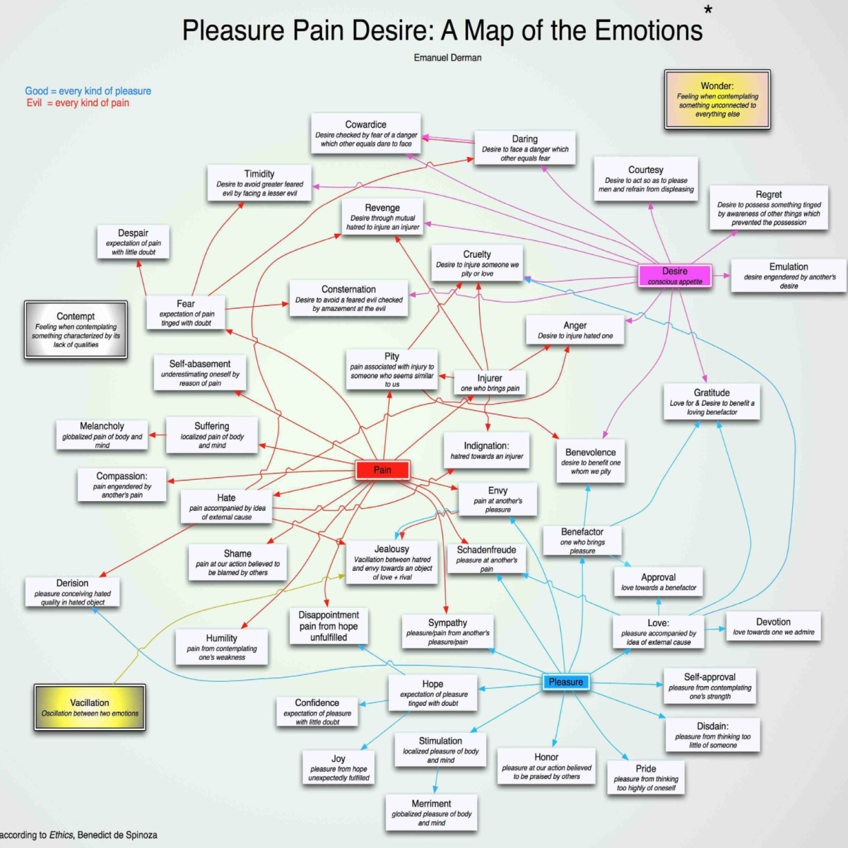
Spinoza developed a system of explaining and defining the passions in terms of their relation to three more primitive feelings: Pain, Pleasure, and Desire. Every passion or emotion, in his view, is a derivative of these three sensations, which lie beneath every passion that Spinoza can name. Thus Hate, for example, is the Pain associated with an external object or person, while Love is Pleasure accompanied by the idea of an external cause.

Some passions have two underliers. Envy is Pain at someone else’s Pleasure, analogous to a convertible bond that depends on both equity and interest rates. Similarly, to give a more com- plex example, Spinoza regards Cruelty as the Desire to inflict Pain on Someone You Love, a triple derivatives analogous to a convertible bond that is additionally exposed to credit risk.

Spinoza, three hundred years before his time, understood derivatives, but his scheme and defi- nitions are virtually static. I say ‘virtually’ because, to be fair, Spinoza does allow for fluctua- tions between passions. He refers to Vacillation, which he defines as the cyclic alternation between two different passions. Thus, for example: Jealousy is the Vacillation between Hatred and Envy in relation to a Love object and a rival. So Vacillation does describe a kind of volatility – the more rapidly and intensely one Vacillates, the greater the Jealousy.

2. The Idea of Diffusion, but without Derivatives
In the 19th Century physicists began to analyze the diffusion of gases.
Thomas Graham in 1831-33: “…gases of different nature, when brought into contact, do not arrange themselves according to their density, the heaviest undermost, and the lighter upper- most, but they spontaneously diffuse, mutually and equally, through each other, and so remain in the intimate state of mixture for any length of time.”

Wikipedia: “In 1858, Rudolf Clausius introduced the concept of the mean free path (the aver- age distance traveled between collisions that characterize the diffusion). In the same year, James Clerk Maxwell developed the first atomistic theory of transport processes in gases. The modern atomistic theory of diffusion and Brownian motion was developed by Albert Einstein, Marian Smoluchowski and Jean-Baptiste Perrin. Ludwig Boltzmann, in the development of the atomistic backgrounds of the macroscopic transport processes, introduced the Boltzmann equation, which has served mathematics and physics with a source of transport process ideas and concerns for more than 140 years.”

So physicists understood diffusion the particles that comprise gases but never applied the idea to functions (i.e. derivatives) of the diffusing substances. They discussed the behavior of underliers, but not functions of underliers.

The exception is of course Bachelier, in this thesis on speculation in France. In the opening year of the 20th Century he developed and applied the theory of diffusion to finance and derived the equations for Brownian motion. He applied them to options with underliers that undergo arithmetic Brownian motion. Far ahead of his time, his work was only rediscovered by the finance community in the 1960s.

3. The Definition of Risk  as Standard Deviation of Returns
In the 1950s, Markowitz applied statistics to highlight the tension between risk and return, with risk measured as the standard deviation of returns. Assuming a knowledge of the future distribution of returns for each stock, he found the portfolio with the most expected return  for a given standard deviation  , or with the least standard deviation for a given expected return.

4. The Idea of Replication as a Strategy for Valuation. (If you like your leverage you can keep your leverage)
1958: Modigliani and Miller showed that the value of a firm is independent of its leverage: You can recreate a levered firm for yourself by borrowing money yourself (rather than the firm levering itself) to buy the stock of an unlevered firm. You will then have created the levered firm for yourself, and it still has the same value.

6. Finance in One Sentence
Richard Feynman was asked for one sentence to leave to posterity from which our knowledge of physics could be reconstructed if all other knowledge of it were lost. His answer was “Everything is made out of atoms.” (I have since heard that there is an equivalent sentence for medicine: “Dis- ease is caused by germs.”) Here is my one sentence to recreate all of financial theory:

IF
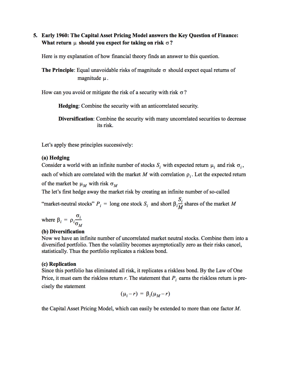
you can hedge away all correlated risk of a security
AND
you can then diversify over all remaining uncorrelated risks
THEN
you should expect only to earn the riskless rate

7. Why is the Capital Asset Pricing Model bad?
Because risk is not as simple as the standard deviation of returns.
Because the market M and the stock S are not really stably correlated.?
Markets are not exactly like flipping coins. Markets depend on psychology, coins don’t. There isn’t a well-defined probability of a market crash.

8. Option Models in the 1960s involve Volatility but no Replication
Various people (Samuleson, Sprenkel, Ayres, Boness …) developed models of derivatives that are actuarial in that they define the value of an option as the expected discounted value of its payoffs. This value does of course depend on the volatility of the stock. But they don’t know what rate of return to use for growing the stock price into the future, and they don’t know what rate to use for discounting the payoffs.
People who wanted to use this model had to forecast the return of the stock and figure out what discount rate to use as a consequence of its risk. It was personal.

9. Black-Scholes and Merton (1971-3): The Combination of Derivatives, Volatility, Hedging and Replication in one Package.
Use diffusion for the underlying stock price
Hedge to eliminate stock risk from option
Require that hedged portfolio, which is riskless, earns the known riskless rate.

Then we get the same formula for the option value as the actuarial one, but where all growth and discount rates are riskless rates.

The value of the option does not depend on the expected return of the stock, since that has been hedged away. Instead it depends on the riskless rate, which is known, and on the future volatility of the stock.

10. Why does option theory work better than CAPM?
Because you really can hedge an option with a stock, because their correlation is really close to 1. So even if you don’t believe that risk is the standard deviation of returns, the two securi- ties really are deeply connected, more deeply than two stocks are to each other.

11. 1970s: Using the Black-Scholes Equation
Now, instead of forecasting the return of the stock, traders must forecast the volatility of the stock.
Black and Scholes set about calculating the “correct” value of an option by using historical volatilities to estimate future volatilities. But who knows what future volatility will be?

12. Calibration: The Discovery of Implied Volatility (1976)
Latane and Rendelman suggest fitting option market prices to the Black-Scholes formula and extracting the WISD (weighted implied standard deviation of the stock). They then suggest calculating hedge ratios from the model using the WISD.
But implied volatilities are unstable.
This process must be repeated as the implied volatility keeps changing from moment to moment, so there is something not quite right.

Implied volatilities tell you that if you believe the model, then, given an option price, this is what the future must be like. But its estimate of the future behavior of the underlier keeps changing.
Nevertheless, from now on everyone calibrates models.
Most people don’t even realize that calibration was an invention.

13. Volatility as an Asset Class
Implied volatility is an estimate of future volatility.
Black-Scholes-Merton say that if you know the future volatility, you can replicate an option, and therefore value it.
But the estimate keeps changing.
So you can’t really replicate: instead you can speculate on volatility, using options.

If you use the model, and hedge the option, an option now become a way of trading volatility rather than a way of speculating on the stock.
In the future: Volatility as an asset class; Variance swaps.

14. 1987: The Appearance of the Smile
Until 1987, options on the same stock with the same expiration but with different strikes all had roughly the same implied volatility. Thus, even though the implied volatilities changed every day, at least they all moved up or down together for different strikes.

After the 1987 crash, low-strike index options have higher implied volatilities than higher- strike options.

When you fit the model to different option strikes, each one implies a different future volatility for the underlying stock. But in the model a stock can only have one volatility. Now some- thing is really wrong – the BS model can NOT accommodate different volatilities for the same stock.

Nevertheless, people keep using the model inconsistently to estimate hedge ratios as they fit it to a given option.

15. 1994 – … The Smile
Extensions of the idea of diffusion: local volatility, stochastic volatility, jumps …

More complexity without true knowledge of the parameters
More calibration: we use the market to imply the model’s parameters – e.g. the volatility of volatility in a stochastic volatility model.

But markets change and these implied parameters are themselves unstable and random, though there are now more of them.

So now, using the stochastic volatility model as an example, you have a market for trading volatility of volatility.

Practitioners and academics develop consistent extensions of Black-Scholes that attribute one process to the underlying stock, but it’s not geometric Brownian motion with a fixed volatility, but rather more complicated processes: e.g. local volatility or stochastic volatility.

16. The Future?
An infinite regress of models?

Each model is inadequate, introduces new parameters, which, as the model is embraced, become random quantities the market can speculate and trade on.

Derivatives are not really derivative, except at expiration.

It takes all of these securities — stocks, options, options on options, volatility, volatility of volatility … to define the possibilities of the market.

Source: Emanuel Derman